Appendix B: The Doppler Effect

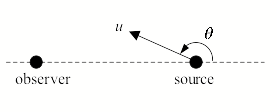
The observed frequency ν′ of light emitted from a source moving with velocity u as depicted in Fig. B1 is given by [4]

                                                  ,                                     (B1)

where ν is the frequency of the light in the rest frame of the source, and c is the speed of light, 299,792  km/s.

Fig B1Geometry of a moving source.  If the source is receding, the measured frequency will be decreased (“red shifted”), compared to the frequency in the rest frame of the source.  If the source is approaching, the measured frequency will be increased (“blue shifted”).  Eq. B1 gives the relationship between the frequencies in the two reference frames.

If the velocity is purely radial, then Eq. B1 reduces to

                                                          ,                                             (B2)

where β² = (c-u)/(c+u).  Note that in Eq. B2 we have adopted the convention that u > 0 indicates a receding source. For our application, we assume the velocity is purely radial (θ= 0° or 180°) and use Eq. 2.[5]  The magnitude of the Doppler effect for some typical situations is given in Table B1.

Table B1Examples of Doppler shifts for 1000 cm-1 (10 μm) light
source	recession velocity (km/s)	shift (cm-1)
geostationary satellite	3	0.01
low Earth orbit satellite	7	0.02
orbital speed of Earth	30	0.1
typical star	300	1
most distant galaxy	75,000	225

Eq. B2 gives the Lorentz transformation for a monochromatic frequency ν.  However, for a continuous spectrum, we cannot simply scale all frequencies.[6]  We must also apply the Lorentz transformation to the (necessarily finite) aperture collecting the radiation.  An aperture subtending solid angle Ω in the rest frame of the source will appear to have solid angle

                                                                                                    (B3)

when receding with velocity u.  Suppose now that the source has a rest-frame radiance of L^P(ν).  An aperture of size Ω  in its rest frame will receive a photon flux of

N(ν) = ΩL^P(ν)

If the aperture is receding with velocity u, the photon flux received from the receding source will be

If the source is a blackbody at temperature T,  (Eq. 4), we have

If we interpret this radiation as coming from a stationary blackbody, that is, L'(ν) = N'(ν)/Ω', then the effective temperature is

                                                              ,                                                  (B4)

Thus the spectrum of a receding blackbody appears identical to a cooler, stationary blackbody.